概要

　ベイジアンネットワークは、ディープラーニング(深層学習)等とは違い変数間の因果関係を捉える事が出来るため、病気の原因分析、気象予測、マーケティングなどで活用されています。今回は、カリフォルニア大学アーバイン校(UCI)が提供しているポルトガルの学生の成績データを使用して、ベイジアンネットワークの構築、評価、介入のシミュレーションを行いました。

CausalNexのインストール方法

今回使用するPythonの因果分析ライブラリCausalNexは以下のコマンドでインストールできます。

$ pip install causalnex

Python3.6~3.8で動きます。(今回はPython3.8.9を使用しています)
プロジェクト毎に仮想環境を立ち上げることが推奨されています。

用語解説

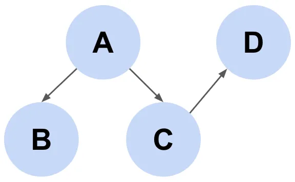
DAG(有向非巡回グラフ)

DAG(有効非巡回グラフ)とは、矢印で繋がれており、循環しないという意味です。つまり、矢印で繋がれている変数間で因果関係を持ち、必ず終端を持つグラフのことです。
*それぞれの変数をノード、ノード間のつながりをエッジと言います。

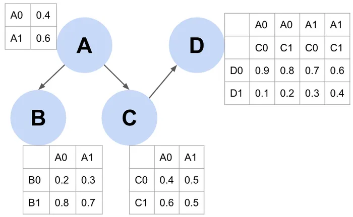
ベイジアンネットワーク

　ベイジアンネットワークとは、ノードが確率変数、エッジが確率変数間の関係を表すDAGと、それぞれの確率変数に関連する条件付き確率分布から構成されるものです。また、下図において、Aの確率テーブルは単にAの確率を表していますが、B,C,Dの確率テーブルは、条件が与えられた場合の確率を表しています。

データ概要

データはstudent.zipにあるstudent-por.csvを使用します。データに存在する項目と意味は以下です。(こちらより引用)

school – student’s school (binary: ‘GP’ – Gabriel Pereira or ‘MS’ – Mousinho da Silveira)
sex – student’s sex (binary: ‘F’ – female or ‘M’ – male)
age – student’s age (numeric: from 15 to 22)
address – student’s home address type (binary: ‘U’ – urban or ‘R’ – rural)
famsize – family size (binary: ‘LE3’ – less or equal to 3 or ‘GT3’ – greater than 3)
Pstatus – parent’s cohabitation status (binary: ‘T’ – living together or ‘A’ – apart)
Medu – mother’s education (numeric: 0 – none, 1 – primary education (4th grade), 2 – 5th to 9th grade, 3 – secondary education or 4 – higher education)
Fedu – father’s education (numeric: 0 – none, 1 – primary education (4th grade), 2 – 5th to 9th grade, 3 – secondary education or 4 – higher education)
Mjob – mother’s job (nominal: ‘teacher’, ‘health’ care related, civil ‘services’ (e.g. administrative or police), ‘at_home’ or ‘other’)
Fjob – father’s job (nominal: ‘teacher’, ‘health’ care related, civil ‘services’ (e.g. administrative or police), ‘at_home’ or ‘other’)
reason – reason to choose this school (nominal: close to ‘home’, school ‘reputation’, ‘course’ preference or ‘other’)
guardian – student’s guardian (nominal: ‘mother’, ‘father’ or ‘other’)
traveltime – home to school travel time (numeric: 1 – <15 min., 2 – 15 to 30 min., 3 – 30 min. to 1 hour, or 4 – >1 hour)
studytime – weekly study time (numeric: 1 – <2 hours, 2 – 2 to 5 hours, 3 – 5 to 10 hours, or 4 – >10 hours)
failures – number of past class failures (numeric: n if 1<=n<3, else 4)
schoolsup – extra educational support (binary: yes or no)
famsup – family educational support (binary: yes or no)
paid – extra paid classes within the course subject (Math or Portuguese) (binary: yes or no)
activities – extra-curricular activities (binary: yes or no)
nursery – attended nursery school (binary: yes or no)
higher – wants to take higher education (binary: yes or no)
internet – Internet access at home (binary: yes or no)
romantic – with a romantic relationship (binary: yes or no)
famrel – quality of family relationships (numeric: from 1 – very bad to 5 – excellent)
freetime – free time after school (numeric: from 1 – very low to 5 – very high)
goout – going out with friends (numeric: from 1 – very low to 5 – very high)
Dalc – workday alcohol consumption (numeric: from 1 – very low to 5 – very high)
Walc – weekend alcohol consumption (numeric: from 1 – very low to 5 – very high)
health – current health status (numeric: from 1 – very bad to 5 – very good)
absences – number of school absences (numeric: from 0 to 93)

These grades are related with the course subject, Math or Portuguese:

G1 – first period grade (numeric: from 0 to 20)
G2 – second period grade (numeric: from 0 to 20)
G3 – final grade (numeric: from 0 to 20, output target)

ベイジアンネットワークの構築

　ここからは、ベイジアンネットワークの構築に入っていきます。以下のライブラリを使用しているので必要に応じてインストールしてください。

import numpy as np
import pandas as pd
import matplotlib.pyplot as plt
%matplotlib inline
from sklearn.preprocessing import LabelEncoder

from causalnex.structure import StructureModel
import networkx as nx
from causalnex.structure.notears import from_pandas

from causalnex.network import BayesianNetwork
from causalnex.discretiser import Discretiser
from causalnex.evaluation import classification_report
from causalnex.evaluation import roc_auc
from causalnex.inference import InferenceEngine
from sklearn.model_selection import train_test_split

DAG(有向非巡回グラフ)の構造学習

　DAGの構造をデータから学習するためには前処理が必要です。前処理は以下の2つを行います

不要な変数の削除 – 性別等の構造に含めたくない変数を削除できます。
データを数値に変換 – CausalNexでは、構造学習の際にデータを数値で持っている必要があります。

データの読み込み

data = pd.read_csv('./student/student-por.csv', delimiter=';')

不要な変数の削除

drop_col = ['school','sex','age','Mjob', 'Fjob','reason','guardian']
data = data.drop(columns=drop_col)

データを数値に変換

struct_data = data.copy()
non_numeric_columns = list(struct_data.select_dtypes(exclude=[np.number]).columns)

le = LabelEncoder()
for col in non_numeric_columns:
    struct_data[col] = le.fit_transform(struct_data[col])

前処理が完了したので、実際にデータから構造学習を行います。 (CausalNexではNO TEARSというアルゴリズムを使用して構造学習を行なっています。具体的な中身が気になる方はこちらの論文を読んでみてください。)

sm = from_pandas(struct_data)

fig, ax = plt.subplots(figsize=(16, 16))
nx.draw_circular(sm,
                 with_labels=True,
                 font_size=10,
                 node_size=3000,
                 arrowsize=20,
                 alpha=0.5,
                 ax=ax)
plt.plot()

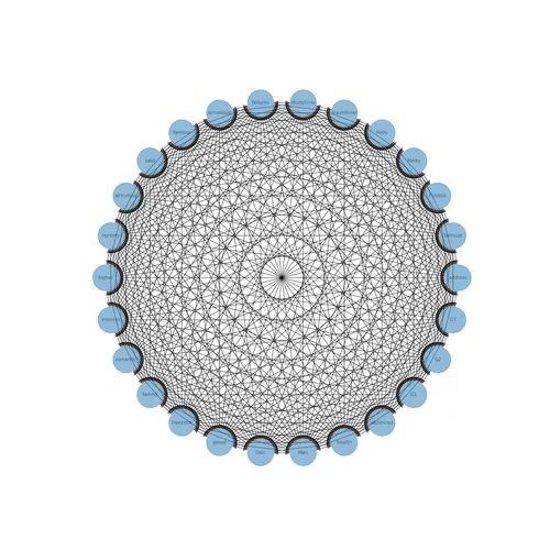
まだ閾値を設定していないので、エッジの数がとても多くなっていますが、閾値を設定することで弱い繋がりのエッジを削除できます。加えて、エッジの太さが繋がりの強さを表すように設定します。

sm.remove_edges_below_threshold(0.8)

edge_width = [ d['weight']*1 <em>for</em> (u,v,d) <em>in</em> sm.edges(data=True)]

fig, ax = plt.subplots(figsize=(16, 16))
nx.draw_circular(sm,
                 with_labels=True,
                 font_size=10,
                 node_size=3000,
                 arrowsize=20,
                 alpha=0.5,
                 width=edge_width,
                 ax=ax)
plt.plot()

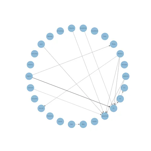
エッジの数は減り、正しそうな因果関係も見えてきています。

Pstatus(両親と一緒に住んでいるか) → famrel(家族関係の質) – 両親と離れて住んでいる場合、家族関係の質が低下する可能性は考えられます。
studytime(勉強時間) → G1(成績) – 勉強時間が長くなると、成績も良くなるはずです。

ただ、正しくなさそうな因果関係も出てきています。

higher(高等教育を希望するか) → Medu(母親の教育水準) – 学生が高等教育を希望するかは母親の教育水準に影響を与えないため、この関係は正しくないです。

正しくないと思われる関係は削除し、加えたい因果関係は追加していきます。また、今回は最大のサブグラフ(DAGが成立しているノードのグループ)のみを使用するのでその部分だけ抽出します

sm = from_pandas(struct_data, tabu_edges=[("higher", "Medu")], w_threshold=0.8)
sm.add_edge("failures", "G1")
sm.remove_edge("Pstatus", "G1")
sm.remove_edge("address", "G1")

sm_l = sm.get_largest_subgraph()

fig, ax = plt.subplots(figsize=(16, 16))
nx.draw_circular(sm_l,
                 with_labels=True,
                 font_size=10,
                 node_size=3000,
                 arrowsize=20,
                 alpha=0.5,
                 width=edge_width,
                 ax=ax)
plt.show()

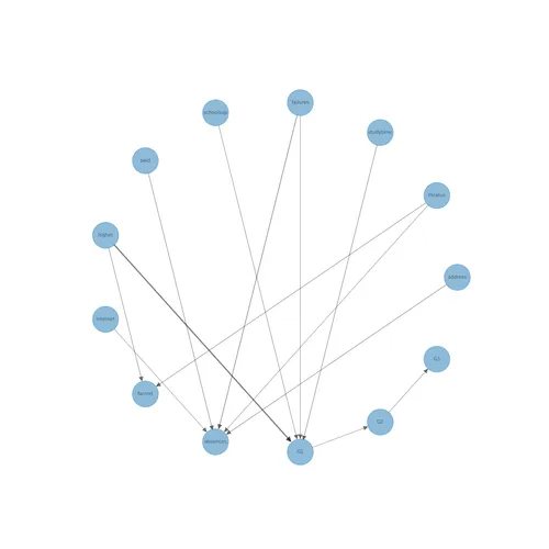
ここまででDAGの構造学習は完了です。

CPD(条件付き確率分布)の学習

DAGの構造学習が完了したので、CPDの学習を行っていきます。 CausalNexは離散分布のみをサポートしているので、離散化処理→CPDの学習と進めていきます。

離散化処理

bn = BayesianNetwork(sm_l)

discretised_data = data[[x <em>for</em> x <em>in</em> sm_l.nodes]]
data_vals = {col: data[col].unique() <em>for</em> col <em>in</em> data.columns}
failures_map = {v: 'no-failure' <em>if</em> v == [0]
                <em>else</em> 'have-failure' <em>for</em> v <em>in</em> data_vals['failures']}
studytime_map = {v: 'short-studytime' <em>if</em> v <em>in</em> [1,2]
                 <em>else</em> 'long-studytime' <em>for</em> v <em>in</em> data_vals['studytime']}
discretised_data["failures"] = discretised_data["failures"].map(failures_map)
discretised_data["studytime"] = discretised_data["studytime"].map(studytime_map)

discretised_data["absences"] = Discretiser(method="fixed",
                          numeric_split_points=[1, 10]).transform(discretised_data["absences"].values)
discretised_data["G1"] = Discretiser(method="fixed",
                          numeric_split_points=[10]).transform(discretised_data["G1"].values)
discretised_data["G2"] = Discretiser(method="fixed",
                          numeric_split_points=[10]).transform(discretised_data["G2"].values)
discretised_data["G3"] = Discretiser(method="fixed",
                          numeric_split_points=[10]).transform(discretised_data["G3"].values)
absences_map = {0: "No-absence", 1: "Low-absence", 2: "High-absence"}
G1_map = {0: "Fail", 1: "Pass"}
G2_map = {0: "Fail", 1: "Pass"}
G3_map = {0: "Fail", 1: "Pass"}
discretised_data["absences"] = discretised_data["absences"].map(absences_map)
discretised_data["G1"] = discretised_data["G1"].map(G1_map)
discretised_data["G2"] = discretised_data["G2"].map(G2_map)
discretised_data["G3"] = discretised_data["G3"].map(G3_map)

CPDの学習

train, test = train_test_split(discretised_data, train_size=0.9, test_size=0.1, random_state=7)
bn = bn.fit_node_states(discretised_data)
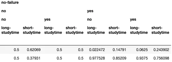
bn = bn.fit_cpds(train)

学習が完了したので、各変数の条件付き確率分布を見ることができます。

bn.cpds["G1"]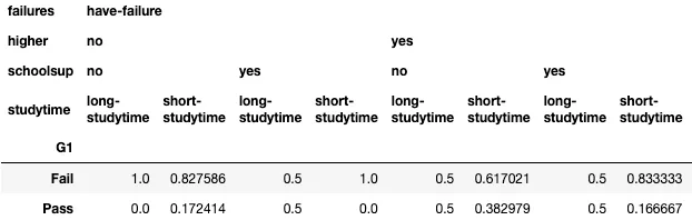

ベイジアンネットワークの評価

　テストデータに対して予測を行ったり、F1スコアやAUCを算出することができます。

とある学生のG1スコアを予測してみました。

predictions = bn.predict(discretised_data, "G1")
print(discretised_data.loc[18,'G1'])

Fail

G1スコアに対して、Precision(適合率)、Recall(再現率)、F1-score(F1スコア)を算出しています。

display(classification_report(bn, test, "G1"))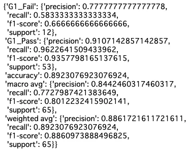

最後に、G1スコアについてのAUCを算出してみました。

roc, auc = roc_auc(bn, test, "G1")
print(auc)

介入のシミュレーション

　CausalNexでは、ある変数が変化した際に確率がどう変わるかをシミュレーションすることができます。例として、学生の100%が高等教育への進学を希望した場合にG1のスコアがどう変わるかを見てみます。

ie = InferenceEngine(bn)

print("G1", ie.query()["G1"])
ie.do_intervention("higher",
                   {'yes': 1.0,
                    'no': 0.0})
print("介入後のG1", ie.query()["G1"])

学生の100%が高等教育への進学を希望した場合に、G1のPassの割合が約74%から約79%に上がる事が推定されました。

まとめ

　今回は、Pythonの因果分析ライブラリCausalNexを用いてベイジアンネットワークの構築、予測や介入のシミュレーションを行いました。構造学習に関してはデータからだけではまだまだ精度が低いのが現実だと思うのでいかにドメイン知識を取り込んでいけるかが重要だと感じました。

参考リンク

SinkCapitalではデータに関する支援を行っています

弊社はスペシャリスト人材が多く在籍するデータ組織です。データ分析や分析基盤の設計などでお困りの方がいらっしゃれば、まずは無料で、こちらから各分野のスペシャリストに直接相談出来ます。

BLOG

Pythonの因果分析ライブラリCausalNexの紹介

概要

目次